
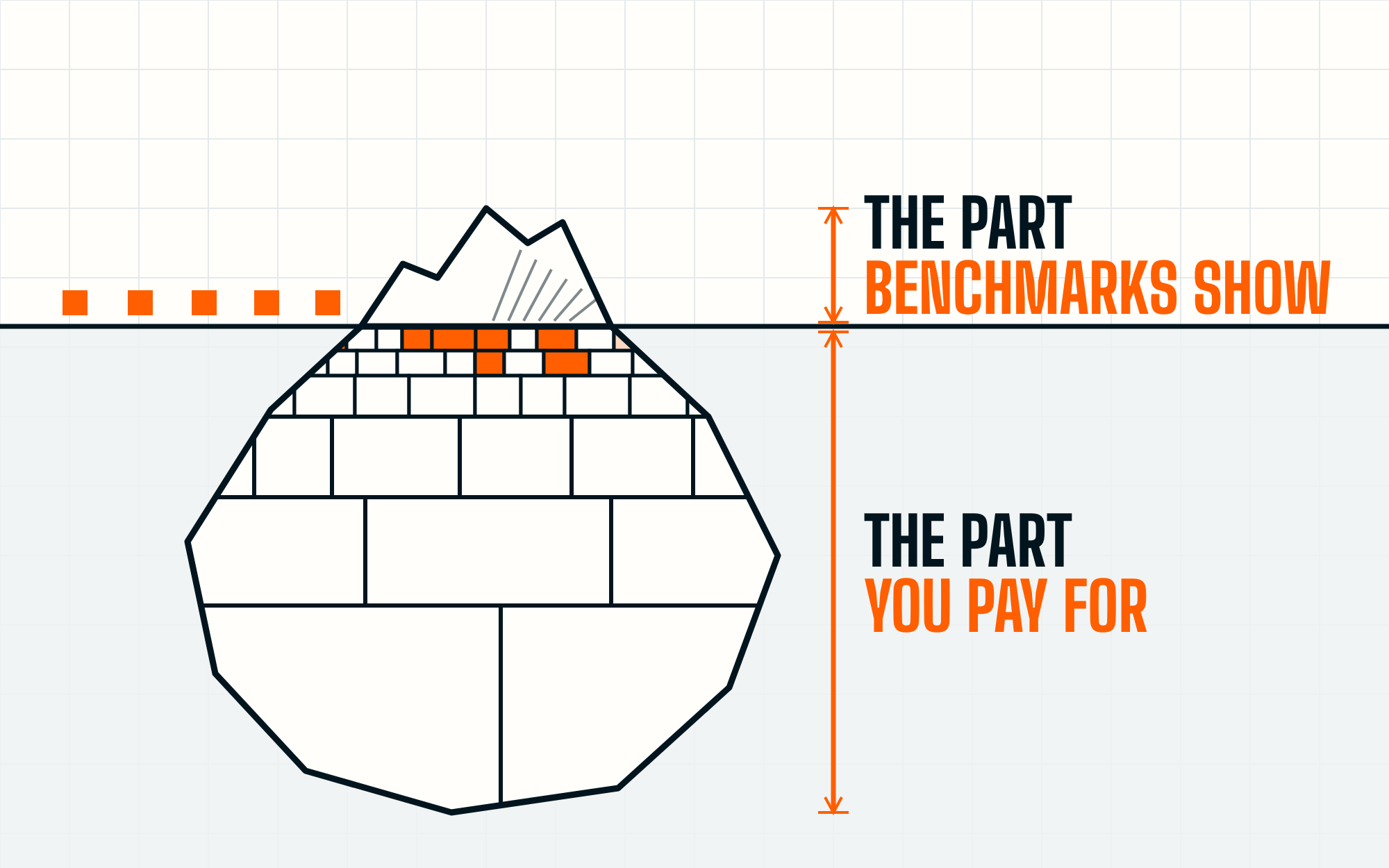
What a fair streaming ingestion benchmark has to measure

Throughput alone won’t tell you whether a table is fresh or what compaction costs. Here’s how we built ingest-bench to measure both, and what it caught.

What a fair streaming ingestion benchmark has to measure
By 
Daniel Liu
Forward Deployed Engineer at Eon
, 
Nov 5, 2026
 • 
0
 min read
How to cite
Liu, D. (2026, November 4). What a fair streaming ingestion benchmark has to measure. The Datamaxxer, Eon. https://www.eon.io/blog/how-to-benchmark-streaming-ingestion

Quick Summary

While building Eon Yukon, we needed to compare how efficiently engines move a continuous stream from Kafka into Apache Iceberg, and the existing benchmarks answered different questions. A throughput number doesn't say whether the table is fresh. An engine's own progress report isn't an independent check. And the compaction that small files create often sits outside the comparison. So we built ingest-bench, and this piece is about how it measures. The results for Yukon, Spark, and Flink are in our benchmark write-up.

Why ingestion deserves its own benchmark

Existing streaming benchmarks address different parts of the problem. NEXMark models an online auction and tests how engines answer continuous queries involving filters, joins, and aggregations, but our workload represents another common use of streaming: getting events into a lakehouse for downstream queries. The emphasis is on writing and committing data, managing partitions, and compaction.

Other benchmarks helped shape our approach. Linear Road, introduced in 2004, asks how many expressways a highway-tolling system can support while answering correctly and on time. It captures an important property of streaming: capacity only counts while the system keeps delivering the required result. LST-Bench examines table formats through writes, queries, and compaction over time. Its treatment of compaction was relevant, but we wanted to compare ingestion engines writing to the same format. We needed to bring these ideas together around the continuous Kafka-to-Iceberg path.

How we set up the test

Fairness starts with the workload. We generate a synthetic corpus and replay the same records on the same schedule for every engine, verifying that Kafka receives the intended load. Our one-hour tests used 200-column Avro events at an offered rate of 1,376 MB/s, about a million rows per second, with both uniform and skewed key distributions. This rate counts encoded values before compression, excluding keys, protocol overhead, and the Confluent header.

We made the corpus configurable so others can test different columns and types, row sizes, key distributions, value ranges, repetition, null frequency, rates, and durations. Kafka partition count and assignment by key or round-robin are configurable too.

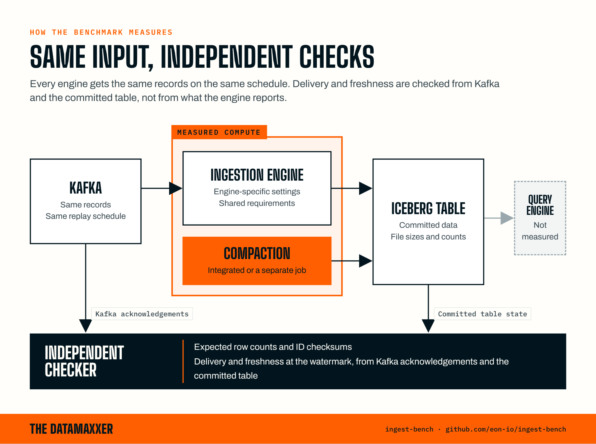
Matching engine settings is less useful than matching the outcome. Different execution and commit mechanisms mean the same interval setting can produce different table freshness. We therefore set a common freshness requirement and let each engine choose how to meet it.

Spark used 40-second micro-batches with adaptive execution. Flink used 60-second checkpoints, with hash distribution for uniform keys and the Iceberg Flink sink's range distribution for skewed keys. We tuned parallelism and memory through probes before the full-hour runs.

For delivery and freshness, we use Kafka acknowledgments and the committed Iceberg table itself, independently of engine-reported progress. Expected row counts and ID checksums let us check the committed output, with a final distinct-ID verification after compaction.
While building Eon Yukon, we needed to compare how efficiently engines move a continuous stream from Kafka into Apache Iceberg, and the existing benchmarks answered different questions. A throughput number doesn't say whether the table is fresh. An engine's own progress report isn't an independent check. And the compaction that small files create often sits outside the comparison. So we built ingest-bench, and this piece is about how it measures. The results for Yukon, Spark, and Flink are in our benchmark write-up. Why ingestion deserves its own benchmark Existing streaming benchmarks address different parts of the problem. NEXMark models an online auction and tests how engines answer continuous queries involving filters, joins, and aggregations, but our workload represents another common use of streaming: getting events into a lakehouse for downstream queries. The emphasis is on writing and committing data, managing partitions, and compaction. Other benchmarks helped shape our approach. Linear Road, introduced in 2004, asks how many expressways a highway-tolling system can support while answering correctly and on time. It captures an important property of streaming: capacity only counts while the system keeps delivering the required result. LST-Bench examines table formats through writes, queries, and compaction over time. Its treatment of compaction was relevant, but we wanted to compare ingestion engines writing to the same format. We needed to bring these ideas together around the continuous Kafka-to-Iceberg path. How we set up the test Fairness starts with the workload. We generate a synthetic corpus and replay the same records on the same schedule for every engine, verifying that Kafka receives the intended load. Our one-hour tests used 200-column Avro events at an offered rate of 1,376 MB/s, about a million rows per second, with both uniform and skewed key distributions. This rate counts encoded values before compression, excluding keys, protocol overhead, and the Confluent header. We made the corpus configurable so others can test different columns and types, row sizes, key distributions, value ranges, repetition, null frequency, rates, and durations. Kafka partition count and assignment by key or round-robin are configurable too. Matching engine settings is less useful than matching the outcome. Different execution and commit mechanisms mean the same interval setting can produce different table freshness. We therefore set a common freshness requirement and let each engine choose how to meet it. Spark used 40-second micro-batches with adaptive execution. Flink used 60-second checkpoints, with hash distribution for uniform keys and the Iceberg Flink sink's range distribution for skewed keys. We tuned parallelism and memory through probes before the full-hour runs. For delivery and freshness, we use Kafka acknowledgments and the committed Iceberg table itself, independently of engine-reported progress. Expected row counts and ID checksums let us check the committed output, with a final distinct-ID verification after compaction.  Freshness must account for data gaps: recent records can appear while earlier ones are still missing. We track the latest point in the stream for which all expected rows have arrived, called the watermark. This watermark tracks complete delivery into Iceberg, rather than progress in event time. Using its Kafka acknowledgment time, we measure how old that point is throughout the run, including between commits. After a five-minute warm-up, our tests required lag to stay within 90 seconds for at least 95 percent of measured time and never exceed 120 seconds. These limits are also configurable. Short probes ruled out configurations that fell behind, and full-hour runs tested promising candidates. We recorded CPU and memory allocations alongside machine types, freshness at each point in time, and the files produced. Test setup The runs shown were conducted October 15 to 22, 2026. Spark 4.1.3 and Flink 2.2.1 used the Iceberg 1.12.0 runtime. Eon Yukon used build 4aae9978. Spark ingestion executors ran on c8gn.4xlarge instances. Yukon and Flink workers, and Spark compaction executors, ran on m8g.4xlarge. Coordinators used m8g.2xlarge, except Flink's maintenance JobManager on m8g.4xlarge. Kafka 4.3.1 ran on six c8gn.8xlarge brokers. The per-run notes document role placement and configuration. What the runs showed about measurement We compared Apache Spark, Apache Flink, and our own Eon Yukon. In the ingestion-only runs, all three engines sustained both workloads and passed our output and freshness checks, at very different allocations. The full numbers are in our benchmark write-up. For method, the useful part is why they differed. The two distributions exposed differences in how engines spread the work. Even with uniformly distributed keys, the busiest writer in our Flink run limited the job while others still had spare capacity. Range distribution spread hot keys in the skewed workload, but its startup phase required more memory for open file writers. Yukon handled both distributions with the same fleet. Key distribution belongs in an ingestion benchmark because the same input rate can place very different demands on the workers. Same workload, different compaction demands Meeting the same freshness requirement could still leave tables with very different file sizes and counts. Our skewed Flink run made this especially clear. While the Iceberg Flink sink's range distribution learned the traffic pattern, it spread unfamiliar keys across writers, producing many small files. The first two commits accounted for 80 percent of the hour's files. Looking only at the settled engine would have missed that work. Compaction is an ongoing part of maintaining a streaming table. A benchmark that leaves it out skips much of the work. Counting compaction changed the comparison. The compute gap between engines moved once maintenance ran alongside ingestion, and Flink's skewed run, which met the freshness limits for ingestion alone, missed them during startup with compaction running. A benchmark that stops at ingestion would miss both. The resulting tables differed too. Yukon consistently produced fewer live files than Spark or Flink. Frequent compaction helped make fresh data query-efficient soon after ingestion by consolidating small files into larger ones. Following rewrite volume, file counts, and compaction duration helped us understand both the compute involved and the state of the table it produced.  A result others can build on A fair comparison of ingestion engines needs to measure throughput, freshness, and correctness alongside the resources required for ingestion and table maintenance. Including our own engine made transparency central to the benchmark. Vendor charts often leave out the details needed to understand what ran. We wanted every result to lead back to its workload, engine version, settings, hardware, compute allocations, and measurements. We also encourage contributors to document why they chose particular settings so that readers can examine the reasoning as well as the configuration. Publishing that detail gives disagreements somewhere useful to go: the workload, configurations, and every run are in ingest-bench. If you're evaluating ingestion engines, ask three questions of any benchmark, including ours. Was freshness measured from the committed table, or from what the engine reported? Was compaction counted, or left for someone else's budget? Were the keys skewed the way your traffic is? A result that can't answer all three is measuring a different job than the one you'll run.

Freshness must account for data gaps: recent records can appear while earlier ones are still missing. We track the latest point in the stream for which all expected rows have arrived, called the watermark. This watermark tracks complete delivery into Iceberg, rather than progress in event time. Using its Kafka acknowledgment time, we measure how old that point is throughout the run, including between commits.

After a five-minute warm-up, our tests required lag to stay within 90 seconds for at least 95 percent of measured time and never exceed 120 seconds. These limits are also configurable. Short probes ruled out configurations that fell behind, and full-hour runs tested promising candidates. We recorded CPU and memory allocations alongside machine types, freshness at each point in time, and the files produced.

Test setup

The runs shown were conducted October 15 to 22, 2026. Spark 4.1.3 and Flink 2.2.1 used the Iceberg 1.12.0 runtime. Eon Yukon used build 4aae9978. Spark ingestion executors ran on c8gn.4xlarge instances. Yukon and Flink workers, and Spark compaction executors, ran on m8g.4xlarge. Coordinators used m8g.2xlarge, except Flink's maintenance JobManager on m8g.4xlarge. Kafka 4.3.1 ran on six c8gn.8xlarge brokers. The per-run notes document role placement and configuration.

What the runs showed about measurement

We compared Apache Spark, Apache Flink, and our own Eon Yukon. In the ingestion-only runs, all three engines sustained both workloads and passed our output and freshness checks, at very different allocations. The full numbers are in our benchmark write-up. For method, the useful part is why they differed.

The two distributions exposed differences in how engines spread the work. Even with uniformly distributed keys, the busiest writer in our Flink run limited the job while others still had spare capacity. Range distribution spread hot keys in the skewed workload, but its startup phase required more memory for open file writers. Yukon handled both distributions with the same fleet. Key distribution belongs in an ingestion benchmark because the same input rate can place very different demands on the workers.

Same workload, different compaction demands

Meeting the same freshness requirement could still leave tables with very different file sizes and counts. Our skewed Flink run made this especially clear. While the Iceberg Flink sink's range distribution learned the traffic pattern, it spread unfamiliar keys across writers, producing many small files. The first two commits accounted for 80 percent of the hour's files.

Looking only at the settled engine would have missed that work. Compaction is an ongoing part of maintaining a streaming table. A benchmark that leaves it out skips much of the work.

Counting compaction changed the comparison. The compute gap between engines moved once maintenance ran alongside ingestion, and Flink's skewed run, which met the freshness limits for ingestion alone, missed them during startup with compaction running. A benchmark that stops at ingestion would miss both.

The resulting tables differed too. Yukon consistently produced fewer live files than Spark or Flink. Frequent compaction helped make fresh data query-efficient soon after ingestion by consolidating small files into larger ones. Following rewrite volume, file counts, and compaction duration helped us understand both the compute involved and the state of the table it produced.
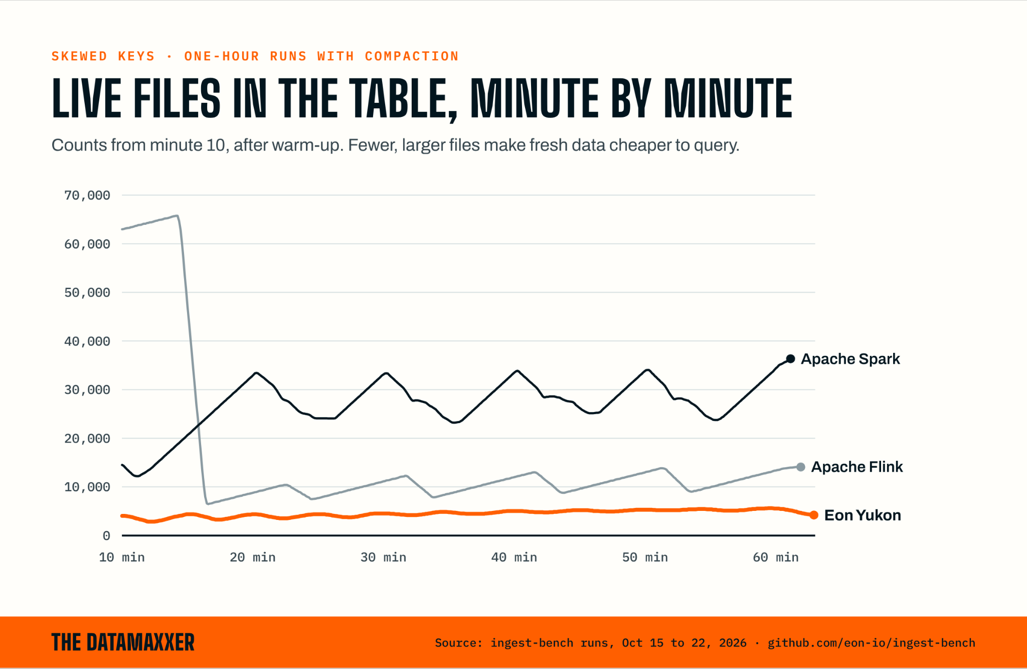
Line chart of live files in the table from minute 10 to 60, skewed keys with compaction. Flink starts above 60,000 files and drops below 10,000 by minute 17, then rises and falls between about 7,000 and 14,000. Spark cycles between about 23,000 and 36,000. Eon Yukon stays between about 3,000 and 6,000.

A result others can build on

A fair comparison of ingestion engines needs to measure throughput, freshness, and correctness alongside the resources required for ingestion and table maintenance.

Including our own engine made transparency central to the benchmark. Vendor charts often leave out the details needed to understand what ran. We wanted every result to lead back to its workload, engine version, settings, hardware, compute allocations, and measurements. We also encourage contributors to document why they chose particular settings so that readers can examine the reasoning as well as the configuration.

Publishing that detail gives disagreements somewhere useful to go: the workload, configurations, and every run are in ingest-bench.

If you're evaluating ingestion engines, ask three questions of any benchmark, including ours. Was freshness measured from the committed table, or from what the engine reported? Was compaction counted, or left for someone else's budget? Were the keys skewed the way your traffic is? A result that can't answer all three is measuring a different job than the one you'll run.

FAQ

No items found.
Daniel Liu
Daniel Liu
Forward Deployed Engineer at Eon

The Datamaxxer newsletter

Hear about it before your boss forwards it to you.

  • 01Tracker updates: every new AI agent and ransomware incident, and whether the data came back
  • 02New research from Eon's engineers, starting with how nine AI models did on a generated company
  • 03Datamaxxing in the wild: real teams getting more out of their data
  • 04One thing to check on your own systems before Monday
See Eon in Action

Cut backup cost and complexity while adding instant restore and analytics.

See Eon in Action

Cut backup cost and complexity while adding instant restore and analytics.